A Brief Respite

Hi Guys,

Thanks for keeping up with my weekly posts!
So, at this point, it's time to start wrapping up my Senior Project.
It's been a truly great experience, and I've learned a lot about it

And, although it's not my last post, and I would not consider this project done yet, here's a link to my SRP presentation here.

Hope you guys enjoy, and keep up for possibly more posts in the near future!

- Alice

Hyperbolic Knots

Hi everyone! It's been a bit of time since my last post, but we'll be catching up on a lot.

In the last two weeks, we went over torus knots and satellite knots. As a brief review, these are, respectively, knots that are wrapped around a torus p times horizontally, q times vertically, and knots that are embedded into other knots. (For details, you can refer to the previous posts here and here.)

We mentioned prime and composite knots a while ago, and we said that composite knots were knots that could be created by composing two nontrivial knots, and prime knots were those that could not.

Interestingly enough, we find that all composite knots are satellite knots, while not the reverse is true. You might wonder: So what about prime knots?

That’s an excellent question, I’m glad you asked! Prime knots are more spread out, but, interestingly, most prime knots are hyperbolic knots. Which, incidentally, is our first topic today!

The formal definition of a hyperbolic knot is “a knot with a complement that can be given as a metric of constant curvature -1”.

What exactly does this mean?

First, let us review the definition of a metric, curvature, etc.

A “metric” is a way of measuring distance between two points. For example, the Euclidean metric is how we usually measure distance between two points, as depicted below (Remember the Pythagorean Theorem?).

In this case, we won’t be using the same Euclidean metric, but a hyperbolic metric.

To understand that, we’ll have to understand curvature. Curvature, much like it sounds, is a measure of much an object “curves.”

Let’s look at the three objects we have below.

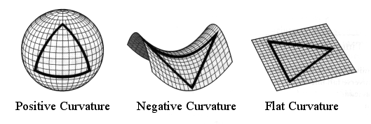Figure 1 - Different kinds of curvature.

Figure 2a - A sphere has positive curvature.

Figure 2b - A saddle-shape has negative curvature.

Figure 2c - A plane has 0 or flat curvature.

Figure 3 - The red is the arc going through the circle with endpoints P1, P2, and the yellow is the segment of the diameter going through P1, P2. (We're pretending here that you have two sets of points P1, P2)

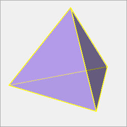Figure 4 - A Euclidean tetrahedron

Figure 5 - A hyperbolic tetrahedron

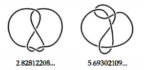Figure 6 - Two different hyperbolic knots with different volumes.

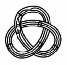
Figure 7 - Two different hyperbolic knots with the same volume

The short answer is just that nobody does it by hand because it takes too long.


References:

If we pick a point on the first sphere shape, we see that if we draw cross sections through it, that all of these curve out in the same direction. Therefore, we say that it has positive curvature.

If we pick a point on the second saddle shape, we do the same to get that the curves are in different directions. Therefore, we say that it has negative curvature

Finally, on the last flat surface, if we attempt to do the same, the cross sections all result in lines. Therefore, we say that this has zero or flat curvature.

Now that we’ve established all of this, let’s go back to our original definition:

the hyperbolic knot is a knot with a complement that can be given as a metric of constant curvature -1.

Here, we have established that, for the complement of the knot, we’ll be using a hyperbolic space, particularly the hyperbolic three-space denoted as H3. Essentially, the points in this, instead of being linear coordinates, are points inside a unit ball, and is denoted as:

Now that we have established our space, we need to find our (nonlinear) distance-measuring metric.

Let us choose two points P1,P2 on the unit sphere. Let us draw a circle going through points P1, P2, where parts of the circle going into the unit sphere are perpendicular. We call arc C the arc of this circle with endpoints P1,P2, such that most of it is inside the unit sphere (aka, the red arc in the figure below).

If points P1, P2 lie on a diameter (any segment going through the center of the circle), then, instead, we let C be the part of the diameter between them (refer to the yellow line in the figure above).

We can then say, that there is only one path that fulfills each of these conditions.

Incidentally, in hyperbolic three-space, the shortest path between two points - let’s call it w for the sake of it - turns out to either be a straight line or an arc of a circle (Hint: one of what we just defined).

These turn out to all be geodesics, which are any arc of a circle or diameter  in H3 that is perpendicular to the unit sphere. Incidentally, if points P1, P2 are on the geodesic, then our path w also falls on this. (Think of it as being the “straight line” of hyperbolic space.)

To measure the distance then, we can’t use the same linear measurement, and, instead, integrate along w (shortest path between P1, P2). Make sense, right? More specifically, it’s defined as 

Now that we have our metric, and our space, we can go back and try to understand what exactly this hyperbolic knot (or even hyperbolic knot complement) seems to be. It turns out, that, to create a hyperbolic knot complement, one takes tetrahedron in hyperbolic space and glues them together.

Usually, in our happy Euclidean space, a tetrahedron looks something like this:

With all that we’ve talked about, the general take-away should be that negative curvature spaces have cross sections that curve in different directions. Therefore, when we put our tetrahedron (pyramid) into a hyperbolic space, it turns into something like this:

We end up taking multiple of these tetrahedron, and gluing the faces together inside H3 (the unit sphere), in order to make a knot complement.

So we’ve found out how to make these hyperbolic knots. How exactly do we distinguish between them? Interestingly enough, we can calculate the volume of these knot complements by adding the volume of the tetrahedron we are gluing together.

Turns out, this is actually an invariant of the hyperbolic knots, known as hyperbolic volume, and any two knots with different volumes must be different knots, for example, the knots below.

Sadly, the inverse cannot be said to be true -- there are (a few) knots with the same hyperbolic volume, that are not the same knot.

At this point, you may be wondering, since we’ve calculated the volume of these hyperbolic knot complements, couldn’t we calculate the volume of these knots? Well, the long answer is that you could, by taking the complement and dividing it into n tetrahedra, which you then get n different equations for, and…

While we could go on all day for hyperbolic spaces and hyperbolic knots, that’s it for hyperbolic knots for now! Thanks for listening, and keep up for the next update!

Abyss.uoregon.edu. N.p., 2016. Web. 14 Apr. 2016.

Loki3.com. N.p., 2016. Web. 15 Apr. 2016.

Mathworld.wolfram.com. N.p., 2016. Web. 15 Apr. 2016.

Adams, Colin Conrad. The Knot Book. New York: W.H. Freeman, 1994. Print.

Knotception (Alternatively, Satellite Knots)

Hello!

Thanks to everyone for keeping up with my knot blog for the past few weeks. 

Last week, we talked about Torus Knots (click  for a quick review! ) and how to create them. This week, we'll be talking about something similar, Satellite Knots. They involve knots inside of other knots (knot sure what that means? read on!), which brings us to the title of Knotception!

Let us consider the Torus shape we talked about last week, and make this a solid (i.e. - An actual donut with everything inside instead of the hollow shell we had before).

We can put a knot K1 inside this torus, so that it is wrapped around the "hole" in the center, see Figure 1. 

Figure 1 - Solid Torus with Knot K1 inside

Now, we can, and this is the fun part, take the torus shell we have, and twist this into the shape of another knot K2, a torus, to be specific. It looks kind of like this:

Figure 2 - A torus twisted into a trefoil.

Except that we still have to remember the knot we had inside the torus. So, it ends up looking something like this:

Figure 3 - The first satellite knot that we have created.

With the 2-dimensional knot inside of the torus. The whole thing, or knot K3, is called a satellite knot, and the knot K2 is called the companion knot of the satellite.

You can think of it, maybe, as knot where the the satellite knot, or the final knot, orbits around (or is inside) the companion torus knot that is the center of the knot as a whole.

Alternatively, we could have an unknot inside the original torus knot. However, though, we have the knot inside twisted around a few times so that it looks as below, and we have the knot and the solid torus together as knot K1.

Figure 4 - The torus, with a knot twisted around inside 

Here, though, if we twist this again into the torus shape as we did before, we have a knot that looks like this:

Figure 5- The Whitehead Knot

We call this a Whitehead Double of a Trefoil (the girl-scout cookie knot shape) because of the original knot's resemblance to the Whitehead link, comprised of two knots and shown below.

Figure 6 - The Whitehead Link. Kind of resembles the knot above.

Now, you may think, where can we go from here.

Well, it turns out, it does matter how we squish the unknot in the middle.

Because if we take the knot we had from before, and, this time, before we twist the torus (donut) into a trefoil (girl scout cookie-shaped knot), we cut it in the middle around the meridian circle (circled in red below), and twist each side around in the direction of the arrows (also shown below) in red.

Figure 7 - Take the knot from before, cut it open across a vertical circle, and twist it around a few times.

We then, take this and twist it, again, into a torus shape, and get the following result.
`

Figure 8 - This is the second Whitehead Double of the Trefoil.

This is a second Whitehead double of the trefoil. Resultingly, the knot inside is called a two-strand cable of the companion knot.

And, on that note, we'll end for this week. Thanks for keeping up, and hope you keep reading for more!

Torus Knots

Hello!

Hope all of you have been having a good week!

This week, We'll be talking about different kinds of knots, not necessarily as classified by an invariant, but known as a Torus Knot.

Before this, though, we should probably explain what a torus is.

The torus, pictured below, is the mathematical equivalent of the outside shell of a donut or bagel, whichever you prefer.

Figure 1 - The Torus

Therefore, a torus knot is a knot that has the knot itself (string), laying on the surface of the torus shape, without crossing over or under itself (i.e. - intersecting itself in any place).

The torus is, incidentally, made up of two types of circles, the meridian curve, which wraps once the short way around the torus, and the longitude curve, which wraps once the long way around the torus.

Torus knots are named as T(p,q), where the knot crosses over the meridian curve (the purple circle in Figure 2) p times, and the longitude curve (the red circle in Figure 2) q times.

Figure 2 - The longitude and meridian curves of the torus. 

An example, would be the (3,5) Torus Knot below in Figure 3. It crosses around the meridian curve five times, while crossing around the longitudinal curve 3 times, and is denoted as the (3,5) torus knot,

Figure 3 - A T(3,5) Knot, or a (3,5) Torus Knot

It's easy to draw a torus knot. For example, for the torus knot (p,q) = (5,3), first, take the torus, and first draw p points, in this case 5 points, on both the inside and the outside meridian curves of the torus, as seen below in Figure 4, in corresponding positions.

Figure 4 - Draw p points on the inside and the outside.

Note how there are two sides of the torus, like the top and bottom has of a hypothetically halved and emptied bagel. To create the Torus Knot, we attach these inside and outside points in different ways.
On the bottom side of the torus attach each of the 5 inside points to each of the 5 outside corresponding points, as shown below in Figure 5.

Figure 5 - On the top half, attach each outside point to the corresponding inside point.

Now, on the top side of the torus, take each outside point, and attach it to the inside point that is a (3/5) clockwise turn, as shown below in Figure 6.

Figure 6 - On the bottom half, attach each outside point to the point that is rotated 3/5th clockwise.

And, now, you've successfully drawn a (5,3) torus knot!

Incidentally, though, we can also show that the knot T(p.q) can be deformed (moved around) to be identical to the knot T(q,p). Essentially, we now know that the T(p,q) and T(q,p) knots are equivalent.

In the diagram below, for example, we see a (3,2) torus knot being transformed into a (2,3) torus knot. It's pretty cool, actually, and makes our job a lot easier - we don't have to keep track of which order to put which in.

Figure 6 - The T(3,2)  Torus Knot is a (2,3)  Torus Knot  

Besides being cool and fun to draw, torus knots important for being relatively simple to classify and look at, and, more specifically, give us a "family" of knots that we can consider at one time. In the papers I'm reading right now, especially, certain statements can be made for torus knots, given their properties, and these specific statements can lead to larger, more interesting generalizations! 

Thanks for reading this week, and hope you keep up for next week's post!

Tricolorability and Reidemeister Moves

Hello, again!


This is the second part of our weekly update, and a continuation of our earlier discussion of tricolorability.

So, essentially, we posed the question of -- can a knot still be tricolorable if you twist it around, poke at it, etc? Why does this matter, you ask.

Well, do you remember how we looked at the unknot last time and pointed out that it can't be tricolorable, because there's no way to color the unknot with at least two colors?


Well, it turns out, if you take the unknot and use a few Reidemeister moves on it, you get this

Figure 1 - The unknot with multiple Reidemeister moves. 

What's to say, then, that one of these later arrangements can't be tricolorable.


Thus, it's useful for us to show that the Reidemeister moves do not affect tricolorability.

Below, then, we can see that each of the Reidemeister moves are not affected by tricolorability
(ie - they remain colorable in at least two colors, and at each of the crossings, have all same or all different colored strands):

Note that, below, as each of the Reidemeister moves are acted upon the section of the knot, the tricolorability (all three colors or only one color) is preserved.

Figure 2a - Reidemeister Move 1

Figure 2b - Reidemeister Move II

Figure 2c - Reidemeister Move III.

Tricolorability, in comparison to other invariants, it is slightly easier to deal with, because if a knot is tricolorable in one projection, then it is tricolorable in any other equivalent projection (i.e. - If you stretch/move/twist it around a lot, it's still tricolorable.)

Thanks for listening, and keep reading for the next post on petal numbers and ubercrossings!

References:

"Figure Eight Knot—Dave Richeson - Math 201: Knot Theory". Math201s09.wikidot.com. N.p., 2016. Web. 5 Mar. 2016.

"Knots | Brilliant Math & Science Wiki". Brilliant.org. N.p., 2016. Web. 5 Mar. 2016.

"The Pretzel Knot - Math 201: Knot Theory". Math201s09.wikidot.com. N.p., 2016. Web. 5 Mar. 2016.

"Tricolorable -- From Wolfram Mathworld". Mathworld.wolfram.com. N.p., 2016. Web. 5 Mar. 2016.

"Unknot". Personal.kenyon.edu. N.p., 2016. Web. 5 Mar. 2016.

Adams, Colin Conrad. The Knot Book. New York: W.H. Freeman, 1994. Print.

Nizami, Abdul Rauf, Mobeen Munir, and Malka Shah Bano. "The Quantum Sl≪Sub≫2≪/Sub≫-Invariant Of A Family Of Knots". AM 05.01 (2014): 70-78. Web. 5 Mar. 2016.

Tricolorability

Hello!

Thanks for keeping up with the blog, and reading up til now.


Today, we'll be talking about two different invariants - Tricolorability, and Ubercrossings and Petal Number.

We'll begin by explaining tricolorability.

So far, with the Reidemeister moves and all of the other invariants we've been talking about, we claim that these are all distinct knots that we can separate from eachother - with the help of these very invariants that we use.

However, how do we know, in the first place, that these knots are all separate. How do we know that some knot that we deem not to be the unknot cannot have a series of Reidemeister moves through which it can become the unknot?

Tricolorability is a clear invariant because, it's obvious.

Remember what a crossing in a knot is? (Hint - It's the place where one piece crosses over another) We call a crossing an undercrossing for the piece underneath, and an overcrossing for the piece above. In a knot projection, the undercrossing will be the piece that is broken up, and the overcrossing will be the one that is continuous.

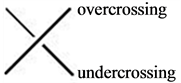Figure 1 - In a crossing, this is the overcrossing and the undercrossing. 

Let us call a strand of a knot the length ranging from one undercrossing to the next.

Now, we can define tricolorability. Do you remember all of those map coloring things where you had to color a map (or just a picture) with 3 or 4 colors? This is similar, in a way.

A knot, or a projection of a knot, is said to be tricolorable if the strands of the knot can be colored so that at every crossing (where 2 or more strands of the knot meet), three different colors or three of the same colors come together. There is, also and interestingly, a rule that a tricolorable knot must be colored with at least two colors.

For example, the trefoil in Figure 2a is obviously tricolorable, but the pretzel knot in Figure 2b would also be tricolorable.

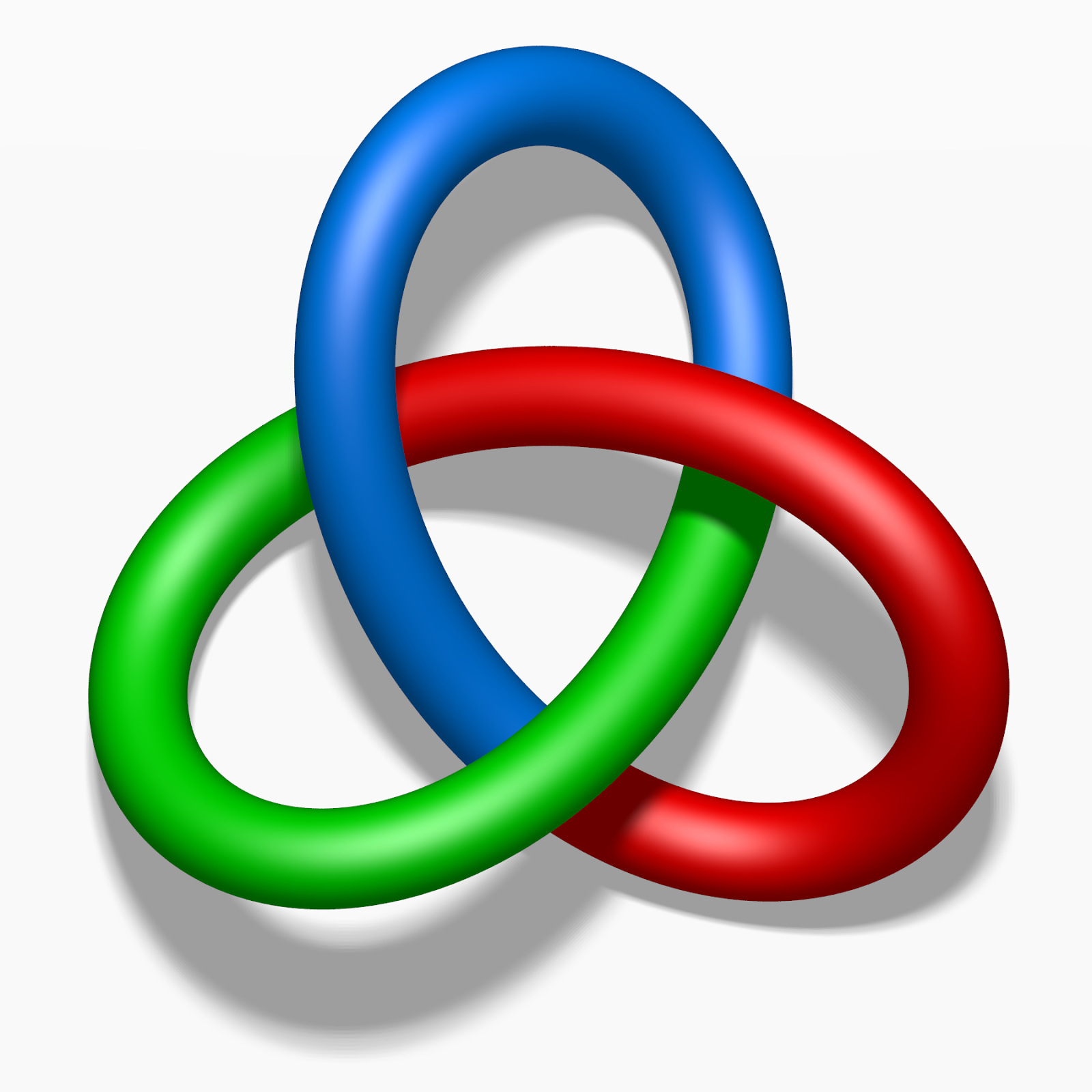Figure 2a - The trefoil is tricolorable. All of its strands are of three different colors at each of the crossings.

Figure 2b- This is the pretzel knot - note that at every crossing, the colors are either all different or all the same.

Alternatively, though, the figure-8 knot and the unknot are both not tricolorable, the unknot (in Figure 3a) for obvious reasons, and the figure-8 knot (in Figure 3b), because it cannot be colored in three colors.

Figure 3a - The unknot is tricolorable because it can only be colored with one color.

Figure 3b - The Figure-8 knot is uncolorable because it cannot be colored with three colors at one crossing.

This invariants gives us a clear distinction between the unknot and the rest of our knots, which proves knot theory to be non-trivial and is helpful for all the work done in it so far.

How do we show that the Reidemeister moves do not affect the tricolorability of the knot, then?

Well, that'll be in the next post - Reidemeister moves and Tricolorability! Keep on reading for more!

Linking back to Links

Continuing on, we talk about the invariant made by links, and the analogous unlink (to the unknot).

Because mathematicians are always very creative people, things get names like as "the unknot" and "the unlink". If you remember the unknot (hint, it's the individual knots on the left and right in Figure 1), the unlink simply consists of two unknots (see Figure 1).

Alternatively, the Hopf link also consists of two unknots, but joined together (see Figure 2).

Figure 1 - The (splittable) unlink is made up of two unknots.

Figure 2 - The (unsplittable) Hopf link is also made up of two unknots.

At this point, you may think, well, it would be nice if we had a way to show exactly how linked two things were. Well, surprise, there is -- and it's called the linking number.

The way to find the linking number is, if you take a 2 component link and designate one as being on the left, and the other being on the right. Then, look at all the places the two cross. If the left one crosses over the right, add one to your total, and if the right one crosses over the left, subtract one from your total (Figure 3).

(+1)

Figure 3 - Calculating Linking Number

Then take this and divide by two. You have your linking number.

If you switch which component is on the left and right, you'll get either the positive or negative of the value. This is an invariant, because, no matter how you twist or turn the knot, the linking number will stay the same.

Unsurprisingly, the linking number of the unlink and the unknot is zero. Also, it is unaffected when the Reidemeister moves (from last week's post) are implemented onto the link.

Anyways, that's it for now. Thanks for keeping up, and see you next week!



References:

Adams, Colin Conrad. The Knot Book. New York: W.H. Freeman, 1994. Print.

Bio.math.berkeley.edu,. N.p., 2016. Web. 27 Feb. 2016.

Exploring Optimal Nutrition,. "Exploring Optimal Nutrition". N.p., 2016. Web. 27 Feb. 2016.

Ndstudies.gov,. "3 - Venn Diagram | North Dakota Studies". N.p., 2016. Web. 27 Feb. 2016.

Upload.wikimedia.org,. N.p., 2016. Web. 27 Feb. 2016.